ASTM D6992 – Accelerated Tensile Creep and Creep-Rupture Testing of Geosynthetics Using the Stepped Isothermal Method (SIM)

27/03/2017ManagerEquipment for Standards, Standards

Introduction

ASTM D6992 is a specialized test method used to determine the accelerated tensile creep and tensile creep-rupture behavior of geosynthetic materials by means of the Stepped Isothermal Method (SIM).

The method is particularly applicable to geosynthetic reinforcement materials such as:

Geogrid ribs
Geotextile strips
Geogrid or geotextile yarns
Single-ply or multiple-ply reinforcement strands
Other narrow polymeric reinforcement specimens where agreement has been established between the concerned parties

The fundamental objective of the method is to obtain information about the long-term deformation and rupture behavior of polymeric geosynthetics without conducting conventional creep tests lasting many years.

The SIM technique accelerates the viscoelastic response of the polymer by subjecting a continuously loaded specimen to a sequence of increasing temperatures. Data from the individual temperature steps are subsequently shifted using the principles of time-temperature superposition to construct a long-term master curve.

ASTM D6992 specifically states that the method may be used to establish sustained-load creep and creep-rupture characteristics. However, results obtained from ASTM D6992 are intended to supplement ASTM D5262 results and should not be used as the sole basis for determining long-term creep or creep-rupture behavior of a geosynthetic material.

1. Principle of the ASTM D6992 Test

Polymeric geosynthetics exhibit viscoelastic behavior. When a constant tensile load is applied to such a material, its strain generally continues to increase with time even though the applied load remains unchanged. This phenomenon is known as tensile creep.

If the applied load is sufficiently high, progressive creep deformation may eventually result in rupture. This behavior is termed tensile creep-rupture.

ASTM D6992 accelerates these time-dependent mechanisms by increasing the specimen temperature in controlled steps while maintaining tensile load.

A typical SIM test therefore consists of:

Establishing the short-term ultimate tensile strength of the material.
Selecting the required creep stress as a percentage of the Ultimate Tensile Strength.
Applying the tensile load to the specimen.
Maintaining the specimen at an initial reference temperature.
Increasing the temperature in predetermined steps.
Maintaining each temperature for a specified dwell period.
Continuously measuring strain, load, temperature, and time.
Rescaling and shifting the individual temperature segments.
Constructing a long-term creep or creep-rupture master curve.

The procedure therefore converts a relatively short laboratory experiment into an estimate of material response over a considerably longer effective time.

2. Important Definitions

Tensile Creep

Tensile creep is the time-dependent deformation occurring while a specimen is subjected to a constant tensile load.

In practical terms:

Constant tensile load + increasing strain with time = tensile creep.

Tensile Creep-Rupture

Tensile creep-rupture is the time-dependent rupture of the specimen while it is maintained under tensile loading.

Higher stress levels are generally used in creep-rupture testing so that rupture occurs within the duration of the accelerated test.

Ultimate Tensile Strength – TULT

The Ultimate Tensile Strength (TULT) is the short-term tensile strength used by ASTM D6992 to normalize the creep and creep-rupture loading levels.

SIM stress levels are consequently expressed as percentages of TULT rather than as arbitrary loads.

For example, if: TULT = 100 kN

and a SIM test is required at: 50% TULT

the target creep load becomes: 50 kN.

The initial tensile test is therefore an essential part of the SIM procedure because subsequent creep loads are derived from its result.

Creep Modulus

Within ASTM D6992 SIM analysis, creep modulus is defined from the applied load relative to the strain at a particular time.

In practical interpretation, the creep modulus provides a measure of the resistance of the material to time-dependent deformation. As creep strain increases under approximately constant stress, the calculated creep modulus generally decreases.

Dwell Time

The dwell time is the period during which the specified conditions are maintained between temperature changes.

During each SIM dwell:

tensile load is maintained,
temperature remains essentially constant,
strain continues to be monitored.

Shift Factor

The shift factor represents the displacement applied along the logarithmic time axis to an individual temperature segment when generating the master curve. It is one of the fundamental parameters involved in time-temperature superposition.

Time-Temperature Superposition

Time-temperature superposition is based on the principle that certain long-term viscoelastic processes occurring slowly at lower temperature can be reproduced more rapidly at elevated temperature.

The creep response obtained at elevated temperatures is therefore shifted horizontally on a logarithmic time axis until individual temperature segments form a continuous master curve.

ASTM D6992 describes the SIM procedure as the use of temperature steps and dwell times to accelerate the creep response of a loaded material.

3. Types of Tests Associated with ASTM D6992

The standard includes three closely related test operations.

3.1 Short-Term Tensile Test

Before SIM testing, tensile testing is performed to determine the Ultimate Tensile Strength, TULT.

The tensile test may additionally provide information concerning:

Elastic strain
Stress-strain response
Secant modulus
Initial strain distribution
Loading behavior

The loading or strain-control conditions used for the tensile test should be the same as, or similar to, those used during the loading ramp of the SIM and Ramp-and-Hold tests.

3.2 Ramp and Hold Test – R+H

The Ramp-and-Hold test is a short-duration creep test.

The specimen is:

Loaded at a predefined rate.
Brought to a predefined tensile load.
Maintained at that load for a relatively short period.

ASTM D6992 describes typical R+H durations on the order of approximately:

100 to 1000 seconds.

The R+H test is particularly useful for determining:

Elastic strain near the end of the loading ramp
Initial rapid creep strain
The transition between immediate and time-dependent deformation

These values may be compared with the initial region of the SIM curve.

3.3 SIM Tensile Creep Test

In the tensile creep version of SIM:

a constant tensile load is applied,
temperature is increased stepwise,
each step is maintained for a controlled dwell period,
strain is recorded continuously.

The purpose is to generate an accelerated long-term creep curve.

3.4 SIM Tensile Creep-Rupture Test

The procedure is fundamentally similar to the creep test, but higher stresses are intentionally selected so that specimen rupture occurs.

Results from several creep-rupture tests may then be used to establish the relationship between:

Applied stress and time to rupture.

This relationship can subsequently be expressed as a regression curve.

4. Test Equipment Required

ASTM D6992 requires a system capable of simultaneously controlling and measuring mechanical loading and environmental temperature.

4.1 Tensile Loading System

Testing may be performed using:

A Universal Testing Machine, or
A dead-weight loading system.

The equipment must provide the functions required for reliable creep testing.

These include:

Load measurement
Load control
Strain measurement
Time measurement
Environmental temperature control
Temperature measurement
Data acquisition

ASTM D6992 specifically identifies computer data acquisition and control as part of the test system capabilities.

4.2 Gripping System

The gripping system is extremely important because an incorrect grip can invalidate creep results.

The grips used for:

Ultimate tensile testing
Ramp-and-Hold testing
SIM creep testing
SIM creep-rupture testing

should be the same or equivalent.

The gripping arrangement must prevent:

Slippage

The specimen must not progressively move inside the grip during the test.

Premature Grip Failure

Excessive localized stress at the grip must not cause rupture before the material itself reaches the intended creep-rupture condition.

ASTM D6992 specifically warns that grips should not initiate failure or cause slippage at stress levels capable of producing specimen rupture.

Before testing, grip surfaces should be checked for:

Dirt
Wear
Damage
Incorrect padding
Loose padding
Surface contamination

4.3 Load Cell

The load cell must:

Have a capacity appropriate for the expected load range.
Be properly calibrated.
Provide sufficient accuracy throughout the intended test range.

An additional consideration in SIM testing is thermal influence on the force-measurement system.

The standard recommends conducting the complete heating program with the apparatus assembled but without a specimen before actual testing.

This thermal verification is intended to determine whether heat transmitted through:

grips,
adaptors,
connectors,
air flow,
structural components,

produces an artificial load-cell signal.

The standard notes that this effect is specific to the particular combination of load cell, grips, adaptors, and fixture configuration.

4.4 Extensometer or Strain Measurement System

The strain-measurement system must be properly calibrated for the expected deformation range.

Potential solutions include:

Contact extensometers
Non-contact optical extensometers
Appropriate displacement transducers

If specimen rupture is expected, the extensometer arrangement should be selected and installed so that rupture does not damage the instrument or create a hazard to the operator.

4.5 Environmental Chamber

The environmental chamber is one of the most important components of an ASTM D6992 system.

The chamber must permit controlled heating and, when necessary, cooling of the specimen.

According to the standard, the chamber/cooling system should be capable of maintaining specimen temperature within: ±1°C

over the range: 0°C to 100°C

and should be capable of changing specimen temperature by as much as: 15°C

within the established ramp time.

Uniform specimen temperature is critical.

It is not sufficient for only the chamber air temperature to reach the target value. The actual specimen must reach thermal equilibrium through its thickness.

5. Sampling Requirements

Specimens used for:

tensile testing,
Ramp-and-Hold testing,
SIM testing,

should all be obtained from the same sample.

This is necessary because the tensile strength used to establish SIM loading levels must be representative of the material undergoing the creep test.

ASTM D6992 requires:

sufficient specimens for the selected tensile test method,
one specimen for each SIM test,
one specimen for each R+H test.

6. Specimen Geometry

Specimen configuration depends upon the type of geosynthetic material.

Geogrids

Geogrid specimens should normally consist of:

one individual rib

unless another configuration has been agreed upon.

Geogrid or Geotextile Yarns

Yarn specimens may consist of:

Single-ply strands
Multiple-ply strands

depending upon the material and agreed test arrangement.

Geotextiles

The standard specifies a nominal strip width of: 50 mm

unless another width has been agreed upon.

The standard notes that narrow strips and individual geogrid ribs are useful because they allow the effect of load on creep properties to be studied separately from specimen-width effects.

However, correlation between narrow specimens and wider representative product specimens should be established when appropriate.

7. Specimen Length and Gauge Length

Overall specimen length depends primarily on the grip system and the tensile test procedure applicable to the material.

For strain measurement, ASTM D6992 specifies, unless otherwise agreed:

Geosynthetic Products

Gauge length = 100 mm

Precursor Yarn Products

Gauge length = 250 to 300 mm

Correct gauge-length definition is essential because strain calculations depend directly upon initial gauge length.

8. Number of Specimens

SIM Creep Master Curve

ASTM D6992 states that a single specimen is usually sufficient for defining a SIM creep or relaxation master curve.

However, where only one SIM test is performed, the onset region of the creep strain or modulus curve should be confirmed by at least:

two short-term Ramp-and-Hold tests.

Creep-Rupture Curve

A considerably larger test population is required for development of a stress-rupture relationship.

The standard indicates that typically: 12 to 18 specimens

are required to establish a stress-rupture curve representing multiple rupture times.

A smaller number can be used when only a limited region of the curve is being investigated.

9. Conditioning and Reference Temperature

The standard reference temperature is: 20 ± 1°C

unless a different reference temperature has been agreed between the concerned parties.

If normal laboratory conditions cannot maintain this range, tensile testing should be performed inside a controlled environmental chamber.

The specimen should remain under the conditioning environment sufficiently long to reach thermal equilibrium.

ASTM D6992 states that this can generally be achieved within several hours, depending on the specimen. Relative humidity must also be recorded for all tests.

10. SIM Test Environment

The standard SIM environment is generally considered a dry environment.

This is important because increasing temperature normally lowers the relative humidity of the surrounding air unless humidity is independently controlled.

The standard reference temperature remains 20°C unless otherwise agreed.

For an individual SIM test, the effective reference temperature is determined from the average temperature achieved during the first isothermal dwell.

11. Temperature Accuracy Requirements

Temperature control is fundamental to the reliability of SIM testing.

The target test temperatures should initially be achieved within: ±2°C of the target temperature.

During an individual temperature step, temperature should then be maintained within: ±1.0°C of the mean achieved temperature.

The specimen must be thermally equilibrated through its complete thickness.

Non-uniform specimen temperature can distort the creep response and make the subsequent shifting procedure invalid.

12. Establishing Thermal Equilibrium

ASTM D6992 suggests the use of calibrated thermocouples positioned:

Near the specimen
Attached to the specimen
Or embedded in the specimen

during preliminary thermal studies.

A sacrificial unloaded specimen may be used to determine how long the material requires to reach the target temperature. The thermocouple should preferably monitor the thickest or most thermally massive part of the specimen.

The time required for this region to achieve the target temperature is then used to establish the minimum practical dwell/ramp condition for testing.

13. Tensile Loading Rate

The loading control used in short-term tensile tests and in the ramp portion of R+H and SIM testing should be the same or similar.

The standard indicates that the loading rate should normally produce a strain rate of approximately: 10 ± 3 %/min

and notes that: 20 ± 3 %/min

is commonly used in European practice.

A constant load-rate does not necessarily produce a constant strain-rate because the stress-strain response of geosynthetic materials is generally nonlinear.

14. Achieving and Maintaining the Target Load

During R+H and SIM testing, the target test load must be accurately established.

The achieved load should be within: ±2% of the target load.

Once established, the achieved load should be maintained within: ±0.5% of its achieved value

throughout the test.

A short load overshoot is permitted if:

it remains within ±2% of the target load, and
its duration is limited to approximately 1–2 seconds.

Replicate loads within a test series should also remain within: ±0.5% of the average achieved load for the test set.

These tolerances are particularly important because creep response is strongly dependent upon applied stress.

15. Pretension and Definition of Zero Strain

Pretension may be applied in accordance with the tensile test governing the material.

However, the laboratory must clearly establish: how zero strain is defined.

The selected zero-strain definition must be reported.

This requirement prevents uncertainty when comparing strain curves from different specimens or laboratories.

16. Specimen Alignment

Before loading, the operator should verify that:

The specimen is correctly positioned in both grips.
The material is aligned with the loading axis.
There is no twist.
The specimen is not laterally offset.
The grip surfaces are clean.
Any grip padding is correctly secured.

Misalignment can introduce bending or uneven stress and produce premature failure.

17. Temperature Step Size

The allowable temperature increment depends strongly on polymer type.

Unless otherwise agreed: Polyester Geosynthetics

Maximum temperature step: 14°C

Polyolefin Geosynthetics

Maximum temperature step: 7°C

The standard provides examples of successful combinations including:

PET: 14°C temperature step with a 10,000 s dwell
HDPE: 7°C temperature step with a 10,000 s dwell

The smaller step for polyolefins reflects their greater temperature sensitivity.

18. Minimum Dwell Time

Unless otherwise agreed, the isothermal dwell period for each SIM step must not be less than: 10,000 seconds

which corresponds to approximately: 2 hours 46 minutes 40 seconds.

For a SIM test that does not end in specimen rupture, the total test duration must normally be at least: 60,000 seconds

or approximately: 16 hours 40 minutes.

A common SIM sequence may therefore consist of approximately six or more isothermal stages.

The example included in the standard’s appendix visually shows stepwise temperature increases over a 60,000-second test period.

19. Typical SIM Test Sequence

A representative practical sequence is:

Step 1 – Determine TULT

Perform the appropriate short-term tensile test.

Calculate:

Ultimate tensile strength
Elongation
Stress-strain relationship

Step 2 – Select SIM Stress Level

Determine the required loading level as a percentage of TULT.

For example:

30% TULT
40% TULT
50% TULT
60% TULT

The actual stress levels depend upon the purpose of the creep or creep-rupture program.

Step 3 – Install the Specimen

Mount the specimen carefully.

Verify:

axial alignment,
correct grip engagement,
gauge length,
extensometer installation,
absence of slippage.

Step 4 – Establish Reference Temperature

Bring the specimen to the reference test temperature.

Normally: 20°C

and allow adequate time for thermal equilibrium.

Step 5 – Apply the Tensile Load

Ramp the load using the specified loading rate until the target creep load is achieved.

Step 6 – Hold the First Isothermal Step

Maintain:

constant load,
reference temperature,

while recording creep strain.

Step 7 – Increase Temperature

Increase chamber temperature by the selected SIM step.

Typical maximum increments are:

14°C for polyester
7°C for polyolefin

unless otherwise agreed.

Step 8 – Stabilize and Continue Monitoring

Once the specimen reaches the new thermal condition, maintain the required dwell period while continuously recording creep response.

Step 9 – Repeat Temperature Steps

Continue successive temperature stages while maintaining the specimen under load.

Step 10 – Complete the Test

The test is terminated when either:

the planned temperature/dwell sequence has been completed, or
creep rupture occurs.

20. Data Acquisition Requirements

Data acquisition rate differs between the loading ramp and constant-load portions.

Initial Loading Ramp

Time, load, and extension must be recorded at a minimum rate of: 2 readings per second.

Constant-Load Period

The minimum recording rate is: 2 readings per minute.

If loading is accomplished using dead weights, regular load measurement after the loading ramp is not required.

Temperature during SIM must be recorded at a minimum rate of: one reading per minute.
A modern ASTM D6992 test system should therefore preferably acquire synchronized channels for:

Time
Force
Extension
Strain
Temperature

throughout the test.

21. Calculation of Tensile Test Results

The first analytical step is calculation of: Ultimate Tensile Strength – TULT

and Elongation

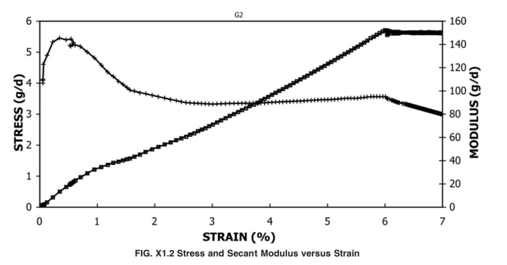
Stress and secant modulus should then be plotted against strain.

ASTM D6992 recommends use of the offset modulus method for normalization or “pointing” of the curves.

The resulting TULT value is then used to calculate the target loading levels for:

R+H testing
SIM creep testing
SIM creep-rupture testing.

22. Ramp-and-Hold Data Analysis

For R+H testing, appropriate plots include:

Stress versus strain
Secant/creep modulus versus strain
Strain versus linear time
Strain versus logarithmic time
Creep modulus versus linear time
Creep modulus versus logarithmic time

The analysis should identify:

Elastic strain at the load-ramp peak
Initial rapid creep strain

These values are used to evaluate whether the initial portion of the SIM response is consistent with short-term material behavior.

23. SIM Raw Data Analysis

For every SIM specimen, initial plots should include:

Stress versus strain
Creep modulus versus strain
Creep strain versus linear time
Creep modulus versus linear time
Stress versus time
Temperature versus time

These plots allow the laboratory to verify whether:

load remained stable,
temperature stages were correctly produced,
strain measurement remained continuous,
unusual events occurred,
specimen slipping occurred,
rupture occurred,
the objectives of the test were achieved.

24. Rescaling the SIM Data

Individual elevated-temperature segments cannot normally be combined directly into a master curve.

They first undergo time rescaling.

The semi-logarithmic slope near the beginning of a higher-temperature dwell is adjusted so that it corresponds with the slope at the end of the preceding lower-temperature dwell.

This is accomplished by subtracting an appropriate time correction from the elevated-temperature dwell data. The purpose is to account for the time consumed by transition and thermal stabilization.

25. Vertical Shifting

After time rescaling, the individual temperature segments may show vertical displacement caused by thermal expansion or other system-related temperature effects.

Vertical shifting is therefore applied to compensate for these effects.

This process improves continuity between adjacent creep or creep-modulus segments.

26. Horizontal Shifting and Construction of the Master Curve

After:

rescaling,
vertical shifting,

the elevated-temperature segments are shifted horizontally along the logarithmic time axis.

They are shifted relative to the initial reference-temperature segment until a smooth continuous master curve is produced.

The final master curve may represent:

Creep Strain vs. Log Time

Creep Modulus vs. Log Time.

ASTM D6992 notes that rescaling and vertical and horizontal shifting normally require iteration to achieve a smooth master curve.

27. Shift Factor Analysis

After completing the master curve, the cumulative shift factors should be determined.

The standard requires preparation of a plot of: Logarithm of cumulative shift factor versus temperature.

This relationship provides important information regarding the time-temperature dependence of the material.

28. Analysis of Creep-Rupture Results

When a series of creep-rupture SIM tests is performed, the results should be plotted as:

Rupture Stress (% of TULT) vs. Log Accelerated Time to Rupture

A linear regression analysis is then performed.

ASTM D6992 specifies that:

time is selected as the dependent variable.

When required, one-sided confidence limits may be calculated at:

90%, or
95%.

The standard also allows determination of an instability strain limit corresponding to the onset of tertiary creep.

29. Primary, Secondary and Tertiary Creep

Understanding the creep stages is useful when interpreting ASTM D6992 data.

Primary Creep

Immediately after loading, creep strain changes rapidly but the rate generally decreases with time.

Secondary Creep

The material reaches a more stable creep-rate region.

This region often dominates long-term service performance.

Tertiary Creep

The strain rate begins to increase significantly.

This stage may indicate:

localized damage,
structural instability,
molecular deterioration,
progressive necking,
or development of failure.

The onset of tertiary creep can therefore be important when establishing an instability strain criterion.

30. Test Validity and Technical Acceptance of the Test Run

It is important to distinguish between:

validity of the laboratory test

and

acceptance of the geosynthetic product.

ASTM D6992 provides a number of measurable requirements that determine whether the SIM test has been performed correctly.

A technically acceptable test should demonstrate, among other requirements:

Correct specimen configuration
Proper axial alignment
No significant grip slippage
No grip-induced premature failure
Calibrated load measurement
Calibrated strain measurement
Correct reference temperature
Adequate specimen thermal equilibrium
Correct loading rate
Correct target load
Required load stability
Correct temperature-step size
Correct dwell duration
Required temperature stability
Sufficient data-acquisition frequency
Valid data shifting
A physically reasonable and continuous master curve
Complete documentation of test conditions

Specific numerical controls include:

Target load: within ±2%

Load during test: within ±0.5% of achieved load

Temperature during a dwell: within ±1°C of mean achieved temperature

Reference temperature: normally 20 ±1°C

Minimum dwell time: normally 10,000 s

Minimum non-rupture SIM duration: normally 60,000 s

Maximum temperature increment: normally 14°C for polyester and 7°C for polyolefins.

31. Does ASTM D6992 Specify a Pass/Fail Requirement for the Product?

This point is particularly important when preparing specifications or certificates.

ASTM D6992 is principally a test-method standard. It does not establish a universal numerical pass/fail limit for all geosynthetic products.

In other words, ASTM D6992 tells the laboratory how to determine accelerated tensile creep and creep-rupture behavior, but it does not state that every geosynthetic must, for example:

remain below a universal maximum creep strain,
achieve a universal minimum rupture time,
maintain a universal minimum creep modulus,
or survive a universally defined percentage of TULT.

Such acceptance criteria must normally come from another governing document, such as:

Product specification
Project specification
Design requirement
Client technical specification
Relevant geosynthetic application standard
Manufacturer’s declared performance
Regulatory requirement

Therefore a product cannot correctly be described simply as “Pass according to ASTM D6992” unless a separate acceptance requirement is also defined.

A technically correct conclusion would instead identify:

The property measured according to ASTM D6992.
The resulting master curve or creep-rupture relationship.
The required design or specification limit.
Whether the measured result satisfies that external requirement.

This interpretation is also consistent with the standard’s stated purpose: SIM creep data are used to predict long-term creep deformation, while creep-rupture data are used to establish the relationship between stress and long-term rupture behavior.

32. Example of Product Acceptance Evaluation

Assume a project specification requires a geogrid to retain sufficient creep-rupture resistance for a specified design lifetime.

The laboratory first generates the ASTM D6992 creep-rupture regression.

The resulting relationship may then be used to determine the predicted rupture strength at the required service time.

For example:

Predicted rupture strength at design life = 42% TULT

If the project specification requires:

Minimum allowable long-term strength = 35% TULT

the product would satisfy that particular project requirement.

However, the 35% limit does not originate from ASTM D6992 unless explicitly stated in another governing specification.

This distinction should always be maintained in technical reports.

33. Test Report Requirements

A comprehensive ASTM D6992 test report should identify the material and test conditions sufficiently to permit technical evaluation and reproduction of the test.

The report should include:

Material Information

Product type
Material type
Brand/trade name
Style or product designation
Structural configuration
Yarn, rib, fabric strip, or other specimen type

Tensile Information

Ultimate tensile strength
Source of tensile-strength value
Whether measured by the laboratory or provided by the manufacturer

Specimen Details

Specimen geometry
Width where applicable
Gauge length
Grip type
Specimen identification
Sampling information

Test Conditions

Reference temperature
Relative humidity
Target load
Achieved load
TULT percentage
Loading rate
Temperature-step sequence
Dwell duration
Total test time

Measurement Information

Load-cell identification
Strain measurement method
Temperature sensor
Data acquisition rate
Calibration status

Results

The report should contain the graphs required by the calculation section, including where applicable:

Stress vs. strain
Creep modulus vs. strain
Creep strain vs. linear time
Creep modulus vs. linear time
Stress vs. time
Temperature vs. time
Rescaled creep curve
Vertically shifted creep curve
Master creep-strain curve
Master creep-modulus curve
Shift factor vs. temperature
Stress-rupture regression

For creep-rupture testing, tabulated rupture values should also be included.

ASTM D6992 requires identification of the tests conducted and the electronic files containing the original test data and requires results generated using the procedure to be identified as having been obtained using the SIM testing protocol of the method.

34. Important Sources of Error

ASTM D6992 is considerably more sensitive to experimental errors than a conventional short-term tensile test.

The most important sources of error include:

Grip Slippage

Even very small movements can be interpreted as creep strain.

Grip-Induced Failure

Stress concentrations may cause premature rupture unrelated to actual material creep strength.

Temperature Gradient Through the Specimen

If the specimen core and surface are at different temperatures, the measured strain cannot be correctly assigned to one isothermal step.

Poor Temperature Stability

SIM relies directly on time-temperature superposition; temperature error therefore directly affects the shift relationship.

Load Variation

Creep is stress dependent, so uncontrolled load changes may significantly affect strain.

Incorrect Zero-Strain Definition

Improper establishment of zero strain can distort the initial section of the master curve.

Inadequate Sampling Rate

The initial loading ramp and transition between temperature steps may contain rapid changes that can be missed by slow acquisition.

Thermal Influence on the Load Cell

Heating of the machine or fixtures may generate apparent force changes even without a specimen.

Incorrect Data Shifting

The final master curve is derived from rescaling, vertical shifting and horizontal shifting. Poor manipulation can create an apparently smooth curve that does not correctly represent the actual material response.

35. Why the SIM Method Is Valuable

Traditional creep and creep-rupture testing may require months or years.

SIM provides an accelerated alternative by combining:

sustained mechanical load,
elevated temperature,
controlled isothermal dwell periods,
time-temperature superposition.

This makes the method particularly useful for evaluation and development of geosynthetics intended for long-term reinforcement applications.

Typical engineering applications include:

Reinforced soil structures
Retaining walls
Embankments
Mechanically stabilized earth systems
Geogrid reinforcement
Long-term load-bearing geotextile applications

36. Relationship Between ASTM D6992 and ASTM D5262

ASTM D6992 should not be regarded as a complete replacement for conventional long-term creep testing.

The standard explicitly states that SIM results are intended to augment results obtained using ASTM D5262 and must not be used as the sole basis for determining long-term creep and creep-rupture characteristics.

Consequently, for critical engineering qualification programs, SIM should normally form part of a broader long-term creep evaluation program rather than being interpreted as an isolated accelerated measurement.

37. Summary of Key ASTM D6992 Test Parameters

Parameter	ASTM D6992 Requirement / Typical Condition
Test type	Accelerated tensile creep / creep-rupture
Method	Stepped Isothermal Method – SIM
Standard reference temperature	20 ±1°C unless otherwise agreed
Geotextile strip width	50 mm unless otherwise agreed
Geogrid specimen	Normally one rib
Geosynthetic gauge length	100 mm unless otherwise agreed
Precursor yarn gauge length	250–300 mm
Normal SIM specimen count	One per SIM test
Confirmation for a single SIM curve	At least two R+H tests
Typical creep-rupture population	12–18 specimens
Typical strain rate	10 ±3 %/min
European practice noted	20 ±3 %/min
Target load accuracy	±2%
Load stability	±0.5%
Replicate load agreement	±0.5% of test-set average
Temperature target achievement	Within ±2°C
Temperature stability	±1°C of mean achieved temperature
Polyester maximum normal step	14°C
Polyolefin maximum normal step	7°C
Minimum dwell	10,000 s
Minimum total non-rupture SIM time	60,000 s
Ramp data acquisition	≥2 readings/s
Constant-load acquisition	≥2 readings/min
Temperature acquisition	≥1 reading/min
Environmental chamber range identified	0–100°C
Primary outputs	Creep strain/master curve, creep modulus/master curve, creep-rupture relationship

Conclusion

ASTM D6992 is an advanced accelerated test method for evaluating the long-term tensile creep and creep-rupture characteristics of polymeric geosynthetic reinforcement materials.

The technique differs fundamentally from a conventional creep test because long-term behavior is reconstructed from a single continuously loaded specimen exposed to a series of controlled isothermal temperature steps.

Successful implementation of the method depends on precise control of:

tensile loading,
strain measurement,
grip performance,
specimen alignment,
specimen temperature,
thermal equilibrium,
dwell periods,
data acquisition,
and subsequent time-temperature superposition analysis.

The most important quantitative requirements include maintaining target creep load within the specified tolerances, maintaining temperature stability within the required limits, using sufficiently long isothermal dwell periods, and collecting synchronized load, strain, temperature, and time data.

For creep testing, the principal result is a long-term creep strain or creep modulus master curve.

For creep-rupture testing, multiple tests are combined to develop a stress versus accelerated rupture-time relationship, which can subsequently be used for long-term engineering assessment.

Finally, ASTM D6992 itself should not be interpreted as establishing a universal product pass/fail threshold. It provides the standardized methodology for obtaining creep and creep-rupture properties. Final product acceptance must be established by comparing these measured properties with the requirements of the applicable project, product specification, design standard, or customer specification.

ASTM D6992 Worked Example – SIM Creep Calculation and Long-Term Prediction

Practical Calculation Example Based on the ASTM D6992 Appendix

The following worked example demonstrates how data obtained from a Stepped Isothermal Method (SIM) test can be processed to calculate creep modulus and subsequently used to construct a long-term creep master curve.

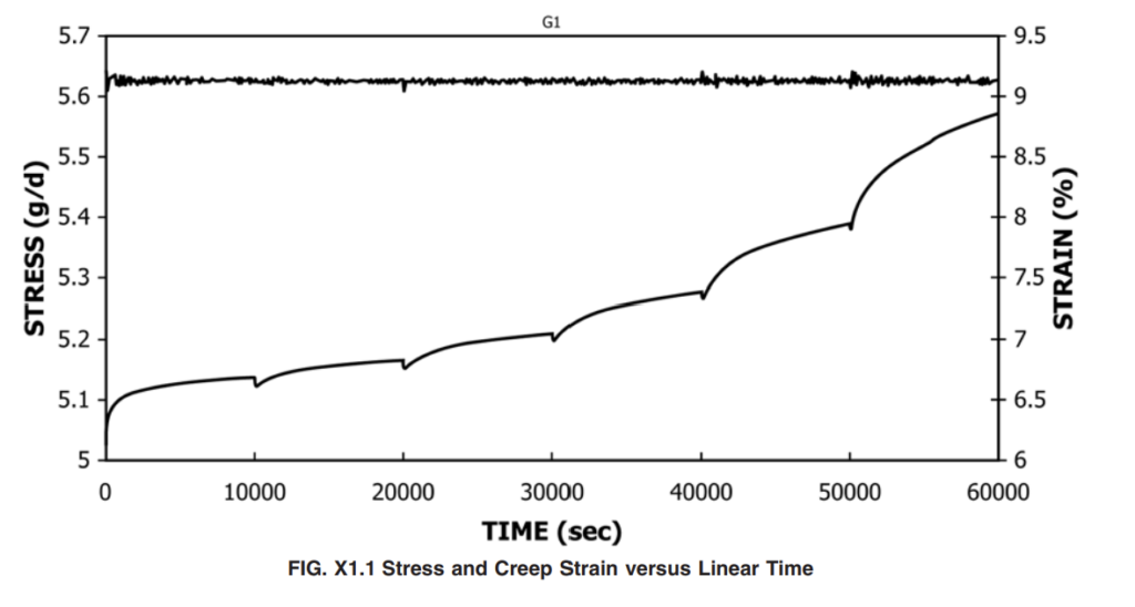
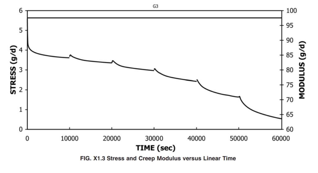
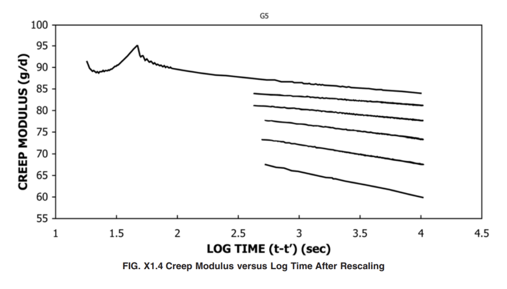
The example is based on Figures X1.1 through X1.8 presented in the Appendix of ASTM D6992-16. These figures show typical results for a polyester yarn before and after rescaling and shifting.

The numerical values used in this example are approximate values read from the ASTM graphs. Therefore, the calculations are intended to explain the ASTM D6992 calculation methodology and should not be considered original laboratory raw data.

The objective of the calculation is to demonstrate the following sequence:

Raw SIM Data → Creep Strain → Creep Modulus → Time Rescaling → Vertical Shifting → Horizontal Shifting → Master Curve → Long-Term Creep Prediction

1. Test Conditions Used in the ASTM Example

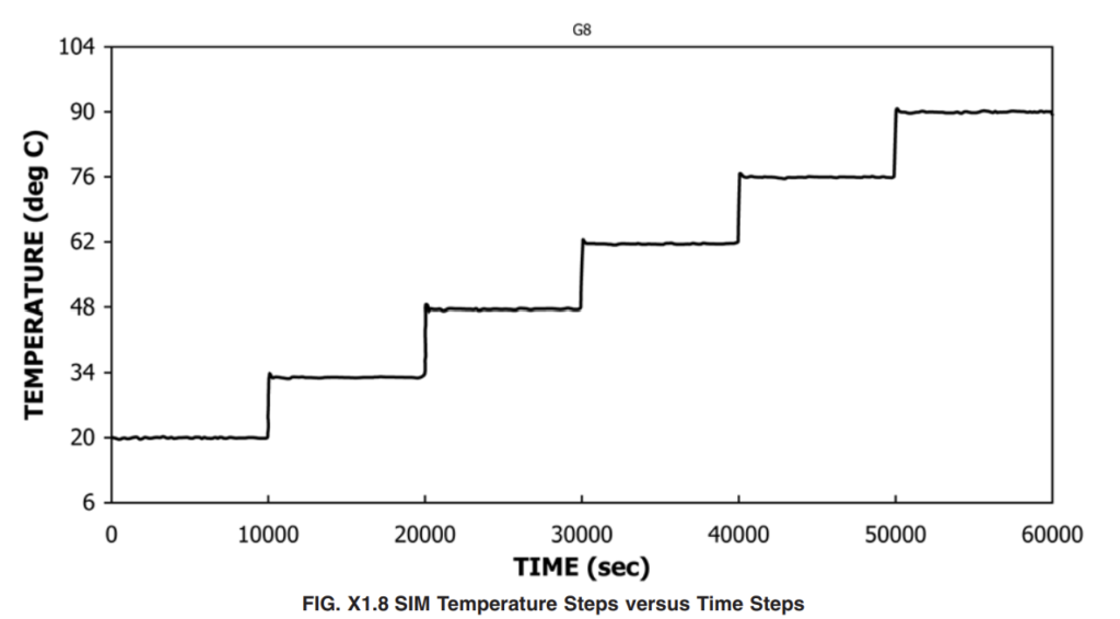
Figure X1.8 shows the temperature history used during the example SIM test.

The physical duration of the test is approximately: 60,000 seconds

which is equivalent to: 16.67 hours

The temperature is increased approximately every 10,000 seconds.

The temperature sequence shown in the ASTM example is approximately:

Physical Test Time	Temperature
0–10,000 s	20°C
10,000–20,000 s	34°C
20,000–30,000 s	48°C
30,000–40,000 s	62°C
40,000–50,000 s	76°C
50,000–60,000 s	90°C

Therefore: Temperature Step ≈ 14°C

and: Isothermal Dwell Time ≈ 10,000 seconds

The physical test therefore consists of six temperature stages. This stepped-temperature program is clearly shown in Figure X1.8 of the ASTM example.

2. Applied Stress During the Test

Figure X1.1 shows the relationship between:

Stress
Creep strain
Physical test time

The applied tensile stress remains essentially constant throughout the test.

From the graph, the approximate stress is: Applied Stress ≈ 5.62 g/d

At the same time, creep strain progressively increases.

Approximate values read from Figure X1.1 are:

Time	Applied Stress	Approximate Creep Strain
10,000 s	5.62 g/d	6.6%
20,000 s	5.62 g/d	6.8%
30,000 s	5.62 g/d	7.0%
40,000 s	5.62 g/d	7.4%
50,000 s	5.62 g/d	7.9%
60,000 s	5.62 g/d	8.8%

This demonstrates the fundamental creep behavior of the polymer:

Constant Tensile Stress + Increasing Strain with Time = Tensile Creep

The raw stress and creep-strain behavior is illustrated in Figure X1.1.

3. Calculation of Creep Modulus

Creep modulus represents the relationship between the applied stress and the strain measured at a particular time.

For the percentage-strain format used in this example:

Creep Modulus = (Applied Stress / Creep Strain) × 100

or:

Mc = (σ / ε) × 100

where:

Mc = Creep Modulus, g/d
σ = Applied Stress, g/d
ε = Creep Strain, %

The multiplication by 100 is necessary because the strain is expressed as a percentage.

4. Creep Modulus at 10,000 Seconds

From Figure X1.1: Applied Stress = 5.62 g/d

and: Creep Strain = 6.6%

Therefore: Creep Modulus = (5.62 / 6.6) × 100

Result: Creep Modulus ≈ 85.2 g/d

Therefore, the estimated creep modulus at 10,000 seconds is:

Mc(10,000 s) ≈ 85.2 g/d

This value is reasonably consistent with Figure X1.3, where the creep modulus around 10,000 seconds is approximately within the range of 84–86 g/d.

5. Creep Modulus at 20,000 Seconds

At approximately 20,000 seconds:

Applied Stress = 5.62 g/d

Creep Strain ≈ 6.8%

Therefore: Creep Modulus = (5.62 / 6.8) × 100

Result: Creep Modulus ≈ 82.6 g/d

6. Creep Modulus at 30,000 Seconds

At approximately 30,000 seconds:

Applied Stress = 5.62 g/d

Creep Strain ≈ 7.0%

Therefore: Creep Modulus = (5.62 / 7.0) × 100

Result: Creep Modulus ≈ 80.3 g/d

7. Creep Modulus at 40,000 Seconds

At approximately 40,000 seconds:

Applied Stress = 5.62 g/d

Creep Strain ≈ 7.4%

Therefore: Creep Modulus = (5.62 / 7.4) × 100

Result: Creep Modulus ≈ 75.9 g/d

8. Creep Modulus at 50,000 Seconds

At approximately 50,000 seconds:

Applied Stress = 5.62 g/d

Creep Strain ≈ 7.9%

Therefore: Creep Modulus = (5.62 / 7.9) × 100

Result: Creep Modulus ≈ 71.1 g/d

9. Creep Modulus at 60,000 Seconds

At the end of the physical SIM test:

Applied Stress = 5.62 g/d

Creep Strain ≈ 8.8%

Therefore: Creep Modulus = (5.62 / 8.8) × 100

Result: Creep Modulus ≈ 63.9 g/d

10. Summary of the Creep Modulus Calculations

The approximate calculated values are summarized below:

Time	Stress	Creep Strain	Creep Modulus
10,000 s	5.62 g/d	6.6%	85.2 g/d
20,000 s	5.62 g/d	6.8%	82.6 g/d
30,000 s	5.62 g/d	7.0%	80.3 g/d
40,000 s	5.62 g/d	7.4%	75.9 g/d
50,000 s	5.62 g/d	7.9%	71.1 g/d
60,000 s	5.62 g/d	8.8%	63.9 g/d

The result clearly demonstrates that creep modulus decreases as creep strain increases.

Figure X1.3 of ASTM D6992 shows the same general behavior: stress remains essentially constant while creep modulus decreases progressively during the stepped-temperature test.

11. Calculation of Creep Modulus Reduction

Using the approximate values calculated above:

Initial Representative Creep Modulus = 85.2 g/d

Final Creep Modulus = 63.9 g/d

The reduction is: Creep Modulus Reduction = 85.2 − 63.9

Therefore: Creep Modulus Reduction = 21.3 g/d

The percentage reduction can be calculated as: Creep Modulus Reduction (%) = (21.3 / 85.2) × 100

Result: Creep Modulus Reduction ≈ 25.0%

Therefore, over the physical SIM sequence considered in this example, the calculated creep modulus decreases by approximately: 25%

This reduction occurs because strain increases while tensile stress remains essentially constant.

12. Why the Six Raw Temperature Segments Cannot Simply Be Connected

The physical test contains six different temperature stages:

20°C → 34°C → 48°C → 62°C → 76°C → 90°C

Each increase in temperature accelerates the viscoelastic creep response of the polyester specimen.

Consequently, the response recorded at 90°C cannot simply be interpreted as a continuation of the response at 20°C on the physical time scale.

The individual temperature segments must first be processed using the time-temperature superposition procedure.

The principal processing stages are:

Time rescaling
Vertical shifting
Horizontal shifting
Construction of the master curve

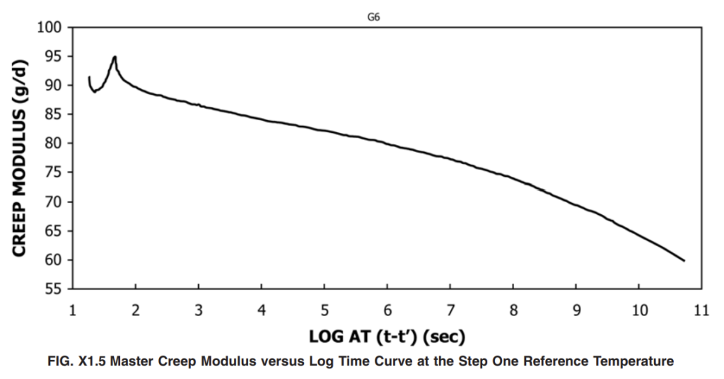
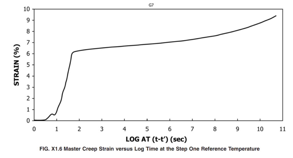
Figure X1.4 shows the individual creep-modulus segments after rescaling, while Figures X1.5 and X1.6 show the final master curves.

13. Time Rescaling

When the temperature changes from one stage to another, the specimen does not instantaneously reach the new isothermal condition. A certain period is required for thermal stabilization. This transition period should not be interpreted directly as normal isothermal creep response.

For this reason, a time correction is applied.

The corrected time can be expressed as: Corrected Time = Recorded Time − Time Correction

or: Corrected Time = t − t′

where:

t = Recorded time
t′ = Rescaling or time-correction value

The resulting corrected time is then used for logarithmic analysis.

14. Simple Example of Time Rescaling

Assume that a data point is recorded: 1,000 seconds

after the beginning of a temperature step.

Assume that the time correction determined during rescaling is: 300 seconds

The corrected time is: Corrected Time = 1,000 − 300

Therefore: Corrected Time = 700 seconds

The logarithmic corrected time becomes: Log Time = log10(700)

Result: Log Time ≈ 2.845

Without the correction: log10(1,000) = 3.000

Therefore, time rescaling changes the horizontal position of the data segment.

The value of 300 seconds in this example is only an illustration of the calculation procedure. The Appendix figures do not provide the complete numerical t′ values used to construct the published master curve.

15. Vertical Shifting

After time rescaling, the individual temperature segments may still show vertical discontinuities.

These discontinuities can result from temperature-related effects such as:

Thermal expansion of the specimen
Thermal expansion of the grips
Fixture expansion
Machine deformation
Extensometer response
Other temperature-dependent displacement effects

Vertical shifting is used to compensate for these effects and improve continuity between adjacent creep segments.

For example, assume that the end of one segment has a creep modulus of: 84.0 g/d

and the beginning of the following rescaled segment gives: 82.5 g/d

The difference is: Vertical Correction = 84.0 − 82.5

Therefore: Vertical Correction = 1.5 g/d

The second segment would therefore require an approximate upward correction of: 1.5 g/d

to establish continuity.

This is an illustrative calculation. The exact vertical corrections applied to the ASTM Appendix data are not numerically tabulated in the figures.

16. Horizontal Shifting and Shift Factor

After rescaling and vertical correction, each elevated-temperature segment must be shifted horizontally along the logarithmic time axis.

The amount of horizontal translation is represented by a temperature-dependent: Shift Factor, AT

Conceptually, the equivalent time can be calculated as:

Equivalent Time = Shift Factor × Corrected Time

or:

Equivalent Time = AT × (t − t′)

This is the fundamental operation that allows a short-duration high-temperature response to represent a much longer response at the reference temperature.

Time-temperature superposition is the central principle behind ASTM D6992 SIM testing. ASTM describes the method as accelerated creep testing using temperature steps and dwell times, with the resulting viscoelastic response shifted along the logarithmic time axis to construct a master curve.

17. Example of a Shift Factor Calculation

Assume that after time rescaling:

Corrected Time = 1,000 seconds

and assume that the shift factor at the elevated temperature is: AT = 1,000

The equivalent time is: Equivalent Time = 1,000 × 1,000

Therefore: Equivalent Time = 1,000,000 seconds

The logarithmic equivalent time is: Log Equivalent Time = log10(1,000,000)

Therefore: Log Equivalent Time = 6

This means that a response physically observed after only 1,000 seconds at the elevated temperature is positioned at an equivalent reference-temperature time of 1,000,000 seconds for this illustrative shift factor.

Again, AT = 1,000 is an example selected to demonstrate the calculation and is not claimed to be the actual shift factor used for a particular segment in the ASTM Appendix.

18. Construction of the Master Curve

After the individual segments have undergone:

Time Rescaling → Vertical Shifting → Horizontal Shifting

they are combined to produce a continuous long-term curve. The final result can be represented as:

Master Creep Modulus vs. Log Time

or:

Master Creep Strain vs. Log Time

Figure X1.5 presents the Master Creep Modulus curve, while Figure X1.6 presents the Master Creep Strain curve at the Step One reference temperature.

The important point is that the master curve is not a simple extrapolation of the original 60,000-second curve.

It is generated by applying time-temperature superposition to the individual isothermal creep segments.

19. Understanding the Logarithmic Time Axis

The horizontal axis of the master curve is logarithmic.

To convert a Log Time value back to seconds: Equivalent Time (seconds) = 10^(Log Time)

For example: Log Time = 6

Equivalent Time = 10^6 seconds

Therefore: Equivalent Time = 1,000,000 seconds

Converting to days: Equivalent Time = 1,000,000 / 86,400

Result: Equivalent Time ≈ 11.57 days

Log Time = 7

Equivalent Time = 10^7 seconds

Therefore: Equivalent Time = 10,000,000 seconds

Converting to days: 10,000,000 / 86,400 ≈ 115.7 days

Therefore: Log Time 7 ≈ 116 days ≈ 0.317 year

Log Time = 8

Equivalent Time = 10^8 seconds

Therefore: Equivalent Time = 100,000,000 seconds

Using approximately 31,557,600 seconds per year: Equivalent Time = 100,000,000 / 31,557,600

Result: Equivalent Time ≈ 3.17 years

Log Time = 9

Equivalent Time = 10^9 seconds

Therefore: Equivalent Time = 1,000,000,000 seconds

Convert to years: Equivalent Time = 1,000,000,000 / 31,557,600

Result: Equivalent Time ≈ 31.7 years

Log Time = 10

Equivalent Time = 10^10 seconds

Therefore: Equivalent Time = 10,000,000,000 seconds

Convert to years: Equivalent Time = 10,000,000,000 / 31,557,600

Result: Equivalent Time ≈ 316.9 years

20. Equivalent Time Table

The logarithmic scale can therefore be interpreted as follows:

Log Time	Equivalent Time
6	11.6 days
7	115.7 days
8	3.17 years
9	31.7 years
10	316.9 years
10.5	approximately 1,002 years

This demonstrates why logarithmic time is particularly useful for long-term creep analysis.

21. Reading Long-Term Creep Strain from the Master Curve

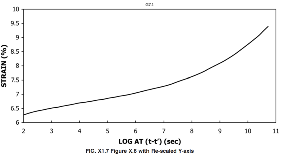
Figure X1.7 provides a rescaled view of the master creep-strain curve.

Approximate graphical readings are:

Log Time	Equivalent Time	Approximate Creep Strain
6	11.6 days	~6.9%
7	116 days	~7.2%
8	3.17 years	~7.6%
9	31.7 years	~8.1%
10	316.9 years	~8.8%

These are approximate graphical readings rather than original electronic data.

Figure X1.7 is specifically presented as a rescaled version of the master creep-strain curve.

22. Prediction of Creep Strain at Approximately 3 Years

Suppose the engineer wants to determine the predicted creep strain after approximately 3.2 years.

First convert time into seconds: Time = 3.2 × 31,557,600

Result: Time ≈ 101,000,000 seconds

The logarithmic time is approximately: Log Time = log10(101,000,000)

Result: Log Time ≈ 8.00

From the ASTM master creep-strain curve at: Log Time ≈ 8

the approximate creep strain is: Creep Strain ≈ 7.6%

Therefore: Predicted Creep Strain at approximately 3.2 years ≈ 7.6%

23. Prediction of Creep Strain at 30 Years

For a design period of: 30 years

convert time to seconds: Time = 30 × 31,557,600

Result: Time = 946,728,000 seconds

Calculate logarithmic time: Log Time = log10(946,728,000)

Result: Log Time ≈ 8.98

This is approximately: Log Time ≈ 9

From the master curve: Creep Strain ≈ 8.1%

Therefore: Predicted Creep Strain at 30 years ≈ 8.1%

24. Prediction of Creep Strain at 50 Years

For: Time = 50 years

convert to seconds: Time = 50 × 31,557,600

Result: Time = 1,577,880,000 seconds

Calculate logarithmic time: Log Time = log10(1,577,880,000)

Result: Log Time ≈ 9.20

From the graphical master curve, the corresponding creep strain is approximately between the values observed at Log Time 9 and 10.

A reasonable graphical estimate is approximately: Creep Strain at 50 years ≈ 8.2–8.3%

This value should be regarded as approximate because it is interpolated from the ASTM graph.

25. Prediction of Creep Strain at 100 Years

For a 100-year design period: Time = 100 × 31,557,600

Therefore: Time = 3,155,760,000 seconds

Calculate logarithmic time: Log Time = log10(3,155,760,000)

Result: Log Time ≈ 9.50

From the master creep-strain curve, the approximate strain at Log Time 9.5 is: Creep Strain ≈ 8.4–8.5%

Therefore, a reasonable graphical estimate is: Predicted Creep Strain at 100 years ≈ 8.5

29. Physical Test Duration Compared with Equivalent Time

Physical SIM test duration: 60,000 seconds

Maximum approximate equivalent time represented graphically: 31,620,000,000 seconds

The ratio is: Time Ratio = 31,620,000,000 / 60,000

Result: Time Ratio ≈ 527,000

Thus, the maximum equivalent time represented by this example master curve is approximately:

5.3 × 10^5 times the physical test duration

This should not be interpreted as a universal SIM acceleration factor.

Each temperature step has its own shift behavior, and the final master curve results from the cumulative time-temperature shifting procedure.

30. Summary of Long-Term Creep Prediction

Using approximate graphical readings from the ASTM Appendix:

Equivalent Time	Log Time	Approximate Creep Strain
11.6 days	6.0	6.9%
116 days	7.0	7.2%
3.17 years	8.0	7.6%
30 years	8.98	8.1%
50 years	9.20	~8.2–8.3%
100 years	9.50	~8.5%
110 years	9.56	~8.5%
317 years	10.0	~8.8%

The ASTM example therefore illustrates how a relatively short accelerated laboratory test can be processed to predict creep deformation over much longer equivalent time periods.

31. Example of an Engineering Acceptance Evaluation

ASTM D6992 itself does not establish a universal creep-strain acceptance limit.

However, the calculated master curve can be compared with an external product or project specification.

For example, assume that a hypothetical engineering specification states: Maximum Permitted Creep Strain at 100 Years = 9.0%

From the ASTM example master curve: Predicted Creep Strain at 100 Years ≈ 8.5%

Compare the two values:

Measured/Predicted Value = 8.5%

Maximum Permitted Value = 9.0%

Since: 8.5% < 9.0%

the material would satisfy this hypothetical project requirement.

The margin relative to the specified limit would be: Acceptance Margin = 9.0 − 8.5

Therefore: Acceptance Margin = 0.5 percentage point

It is essential to emphasize that the 9.0% limit in this example is hypothetical and is not an ASTM D6992 acceptance requirement.

ASTM D6992 provides the methodology for obtaining accelerated creep and creep-rupture properties. Final acceptance criteria must be obtained from the applicable:

Product specification
Project specification
Design standard
Customer requirement
Regulatory requirement

ASTM itself describes creep data from this method as being used to calculate creep modulus as a function of time and to predict long-term creep deformation of geosynthetics used in reinforcement applications.

32. Important Difference Between Prediction and Certification

The long-term values obtained from the master curve should be understood as:

SIM-Based Long-Term Predictions

They are not direct physical measurements performed over 30, 50, 100 or 300 years.

For example: 100-year predicted strain ≈ 8.5%

does not mean that the laboratory physically maintained the specimen under load for 100 years.

The physical test lasted approximately: 16.7 hours

and the long-term response was reconstructed using:

Temperature acceleration
Time rescaling
Vertical shifting
Horizontal shifting
Time-temperature superposition

This distinction is fundamental when reporting ASTM D6992 results.

33. Important Limitation of the ASTM D6992 Method

ASTM D6992 specifically states that SIM results are intended to augment ASTM D5262 results and should not be used as the sole basis for determination of long-term creep and creep-rupture behavior of geosynthetic materials.

Therefore, particularly for critical engineering applications, SIM results should be interpreted together with appropriate conventional creep data and other relevant material-performance information.

34. Complete Calculation Flow

The complete calculation procedure can be summarized as:

Step 1 – Perform the Physical SIM Test

Apply a constant tensile load while increasing temperature in controlled steps.

For the ASTM example:

20°C → 34°C → 48°C → 62°C → 76°C → 90°C

Step 2 – Measure Creep Strain

Record strain continuously during each isothermal dwell.

Step 3 – Calculate Creep Modulus

Use: Creep Modulus = (Applied Stress / Creep Strain) × 100

Example: Creep Modulus = (5.62 / 6.6) × 100

Result: Creep Modulus = 85.2 g/d

Step 4 – Separate Individual Temperature Segments

Divide the raw curve into individual isothermal dwell sections.

Step 5 – Perform Time Rescaling

Use: Corrected Time = Recorded Time − Time Correction

or: Corrected Time = t − t′

Step 6 – Apply Vertical Correction

Correct discontinuities caused by thermal expansion and other temperature-dependent effects.

Step 7 – Apply Horizontal Shift

Use the shift factor: Equivalent Time = AT × Corrected Time

or: Equivalent Time = AT × (t − t′)

Step 8 – Construct the Master Curve

Combine the corrected and shifted segments into a continuous: Creep Strain vs. Log Time

or: Creep Modulus vs. Log Time

master curve.

Step 9 – Convert Required Design Time to Log Time

For example, for 100 years:

Time = 100 × 31,557,600

Time = 3,155,760,000 seconds

Then:

Log Time = log10(3,155,760,000)

Log Time ≈ 9.50

Step 10 – Read the Predicted Creep Property

At: Log Time ≈ 9.50

the example master curve indicates approximately: Creep Strain ≈ 8.5%

Therefore: Predicted 100-Year Creep Strain ≈ 8.5%

35. Final Worked Example Summary

For the polyester yarn example presented in the ASTM D6992 Appendix:

Physical SIM Test Duration: approximately 60,000 s

Physical Test Duration: approximately 16.7 h

Initial Temperature: approximately 20°C

Final Temperature: approximately 90°C

Temperature Step: approximately 14°C

Dwell Time: approximately 10,000 s per stage

Applied Stress: approximately 5.62 g/d

Creep Strain at approximately 10,000 s: approximately 6.6%

Creep Strain at approximately 60,000 s: approximately 8.8%

Calculated Creep Modulus at approximately 10,000 s: approximately 85.2 g/d

Calculated Creep Modulus at approximately 60,000 s: approximately 63.9 g/d

Approximate Creep Modulus Reduction: approximately 25%

Predicted Creep Strain at approximately 3.2 years: approximately 7.6%

Predicted Creep Strain at approximately 30 years: approximately 8.1%

Predicted Creep Strain at approximately 50 years: approximately 8.2–8.3%

Predicted Creep Strain at approximately 100 years: approximately 8.5%

Predicted Creep Strain at approximately 317 years: approximately 8.8%

Maximum Equivalent-Time Range Visible in the Example Master Curve: on the order of 1,000 years

Conclusion

This worked example demonstrates the complete engineering logic behind accelerated tensile creep analysis according to ASTM D6992.

A specimen is subjected to an essentially constant tensile load while the temperature is increased through a series of controlled isothermal steps. The elevated temperatures accelerate the viscoelastic response of the polymer, allowing substantial creep information to be collected within a relatively short physical test period.

The raw strain data are first used to calculate creep modulus. The individual temperature segments are then separated, time-rescaled, vertically corrected, and horizontally shifted according to the time-temperature superposition principle.

The resulting master curve represents creep behavior over a much wider equivalent-time range than the actual physical duration of the test.

In the ASTM Appendix example, a physical test lasting approximately 16.7 hours produces a master curve extending over many orders of magnitude of equivalent time. The curve can subsequently be used to estimate creep strain or creep modulus at engineering design periods such as 10, 30, 50 or 100 years.

However, these long-term values must be interpreted as SIM-based predictions, not direct measurements over the corresponding service period. Furthermore, ASTM D6992 does not establish a universal product pass/fail criterion. Acceptance must be based on the requirements of the applicable product specification, project specification, design standard, or customer requirement.

The method is therefore particularly valuable for evaluating the long-term mechanical performance of geosynthetic reinforcement materials where conventional creep testing over the full intended service life would be impractical.